Author: Guancheng Li of Tencent Xuanwu Lab

In today’s digital world, classical public-key cryptography such as RSA-2048 and ECC are the most widely used encryption standards, supporting the underlying trust of network security, financial transactions, and privacy protection. However, this cornerstone is facing the potential threat of quantum computing. In theory, quantum computers can factorize large integers and solve discrete logarithms at speeds far exceeding classical computers, thereby breaking RSA and ECC encryption in a short time. This prospect is both exciting and worrying.

The question is: what stage has the development of quantum computers reached? Some optimistically believe that the “countdown” to classical public-key cryptography has already begun; others doubt that truly usable quantum computers are still far away due to manufacturing difficulties. There are various opinions in the market, often optimistic or pessimistic, but the core question always lingers: how far are quantum computers from breaking classical public-key cryptography? We will attempt to answer this question by dismantling and analyzing the manufacturing bottlenecks and breakthrough hopes of quantum computers.

We will attempt to answer this question by dismantling and analyzing the manufacturing bottlenecks and breakthrough hopes of quantum computers.
This series is divided into three parts:

Why Can Quantum Computers Accelerate Computation?
How Are Quantum Computers Built?
What Challenges Remain in Building a Quantum Computer Capable of Breaking RSA 2048?

First, to help readers understand the principles of quantum computing, we will introduce necessary quantum mechanics concepts, such as quantum states and entanglement, and explain why quantum computers can achieve acceleration for specific problems; second, to give everyone an intuitive understanding of the form and implementation path of quantum computers, we will analyze their basic construction and focus on dismantling the internal structure of currently fastest-developing and most engineering-feasible superconducting quantum computers; finally, using superconducting quantum computers as an example, we will deeply analyze the bottlenecks they still face in moving toward breaking classical public-key cryptography (RSA-2048), and the potential solutions behind these problems.

Our conclusion is: at the scientific level, there are no “dead ends,” and the real challenges are concentrated in engineering implementation. Cooling, control, wiring, energy consumption, and real-time implementation of quantum error correction remain huge challenges, but with the advancement of scale expansion and modular design, these problems are expected to be gradually alleviated. Considering current trends, we agree with the industry’s general prediction: million‑qubit quantum computers are very likely to appear in the 2030s, at which time the defense line of classical public-key cryptography will most likely be breached. This also means that post-quantum migration work must start as early as possible. On the one hand, the “Store Now, Decrypt Later” attack mode already exists in reality—sensitive data, even if stolen today, may be decrypted by quantum computing in the future; on the other hand, the migration of cryptographic systems itself is a huge project involving algorithm replacement, system transformation, standard compliance, and ecosystem adaptation, usually requiring many years to complete. If we wait until quantum computers are truly about to emerge before taking action, it is often too late.

This article is also published on “科普中国” and “Tencent PQC InfoHub”. The latter site also offers high-quality content such as post-quantum migration guides, tracking of best practices, post-quantum cryptography standards, and algorithm performance benchmarking. Feel free to follow! 👏

Part 1: Why Can Quantum Computers Accelerate Computation?

The core advantage of quantum computers lies in their utilization of quantum superposition and quantum entanglement. To understand why they can accelerate computation, we first need the basic features of quantum physics—superposition, collapse, and entanglement.

Note: To make it understandable for readers unfamiliar with mathematics or physics, this section will try to avoid using mathematical formulas, which may result in some inaccuracies in details, but will not affect overall understanding. For readers with a certain mathematical foundation, you can read alongside Appendix 1, which provides a more intuitive explanation of phenomena such as superposition states, collapse, and entanglement in mathematical form.

Superposition and Collapse

In classical physics, the state of a system (such as position or velocity) is definite at any moment. In quantum mechanics, the situation is different. Before measurement, a particle’s physical quantity (such as position, momentum, spin, or energy level) is not at a specific value, but in a superposition that simultaneously contains all possible outcomes. Only upon measurement does this superposition collapse to a definite value according to a probability distribution.

A simple example: imagine two small boxes, and a particle can only appear in one of them. Classically, it is either in the left box or the right box—never both. Quantum experiments show that before measurement, the particle is in a state that “contains both left and right possibilities.” Only when we actually measure it does the particle appear in one of the boxes. This process is called collapse. During collapse, each possible outcome has a probability (these probabilities sum to 1, and the distribution is an intrinsic property of the superposition). For example, a particle might be in a superposition with:

Probability of appearing on the left is 70%
Probability of appearing on the right is 30%

This may sound incredible, but the existence of superposition states has long been verified through experiments. A classic example is the double-slit interference experiment with electrons. Interested readers can further look up related experiments.

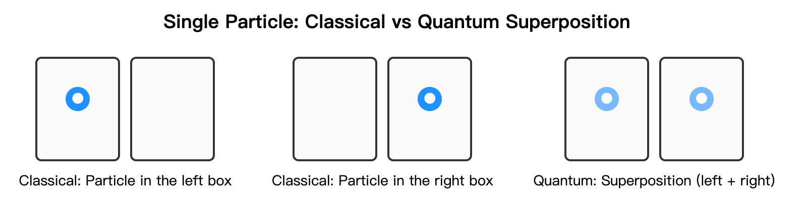
Figure: Classical state vs. quantum superposition. Color indicates measurement probability.

Based on this principle, quantum computers select two clearly distinguishable results from a physical system as the basic unit of information. For example, we can specify “particle in the left box” as 0 and “particle in the right box” as 1. In this way, before being measured, a qubit is not simply 0 or 1, but simultaneously contains both possibilities. When measurement occurs, it will be determined as one of them. This means that qubits can simultaneously carry information of both 0 and 1 in superposition form before measurement, which is the fundamental characteristic that distinguishes them from classical bits.

Quantum Entanglement

After seeing that a single quantity can exist in multiple possibilities via superposition, we can discuss quantum entanglement. Entanglement is a nonclassical correlation: when certain properties (such as position) of two or more particles are entangled, those properties are no longer independent but behave as a single, inseparable whole.

Example: imagine two identical boxes, one on the left and one on the right. Place two particles, labeled 1 and 2. Classically, there are four possibilities, each with some probability:

Both particles in the left box (denoted LL)
Both in the right box (denoted RR)
1 in the left box and 2 in the right (denoted LR)
1 in the right box and 2 in the left (denoted RL)

Classically, the particles are in one definite combination; we just don’t yet know which.

However, in quantum physics, if the two particles are prepared in an entangled state where they must occupy different boxes (an odd‑parity Bell state), then the picture changes. Before measurement, they are not fixed in any specific combination but in a joint superposition. In this state, only two possibilities exist:

1 on the left, 2 on the right (LR)
1 on the right, 2 on the left (RL)

Upon measurement, the system instantly collapses to one of them—either LR or RL. Each outcome has a probability (the probabilities need not be equal; the distribution is an inherent property of the entangled state), while LL and RR occur with zero probability. Thus, quantum entanglement extends the idea of superposition to multi‑qubit bases. Its existence has been confirmed in many experiments (see, e.g., EPR paradox, Bell inequality).

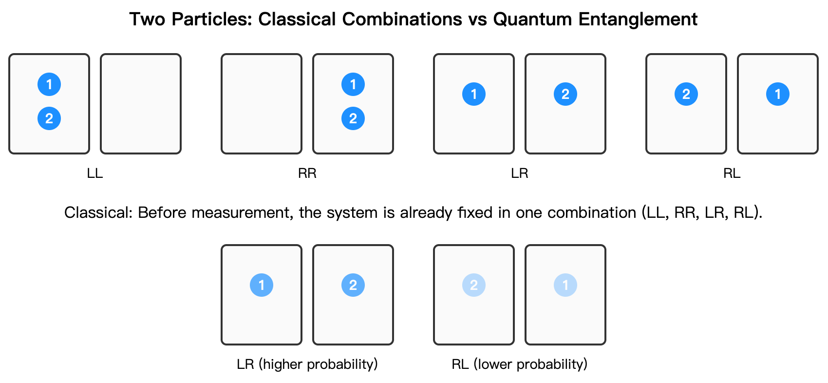
Figure: Classical combinations vs. outcomes from an entangled pair.

Applying this to qubits (e.g., map L→0 and R→1), we can prepare an entangled state where the two qubits always differ. Before measurement, the pair is not definitely “01” or “10,” but a superposition of both. Measurement collapses the state to either “01” or “10,” while “00” and “11” never occur.

Using Superposition and Entanglement to Accelerate Computation

Superposition gives qubits the ability to simultaneously exist in multiple states before measurement, and entanglement allows qubits to form non-classical strong correlations, which are indispensable core resources in many quantum algorithms and quantum error correction.

Here’s an intuitive example. Suppose we have a system of $n$ qubits representing an input variable $x$. By superposition, the state of $x$ can simultaneously cover all values from $0$ to $2^n-1$, not just a single number. Feeding such a state into a function $f(x)$ produces an output that is a superposition of all corresponding results.

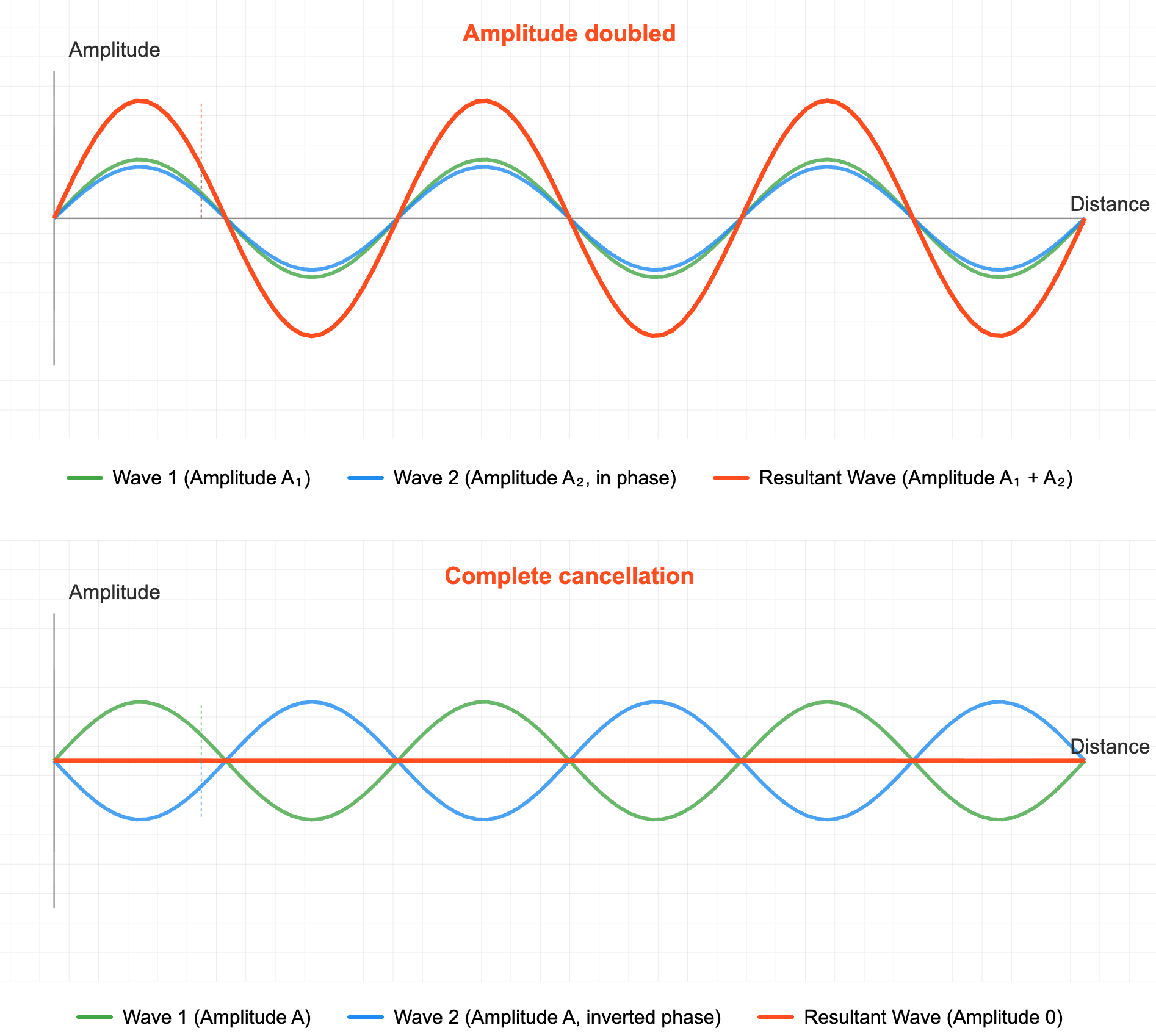
If we want to find the value of $x$ that satisfies $f(x)=c$, we can use carefully designed quantum algorithms (involving the use of mechanisms such as quantum entanglement and quantum interference) to enhance the probability amplitude corresponding to the correct result while weakening the probability amplitude of incorrect results. In this way, during final measurement, we can obtain the correct answer with a higher probability. It should be emphasized that this process of “amplifying the probability of correct solutions” is one of the core ideas of quantum algorithms.

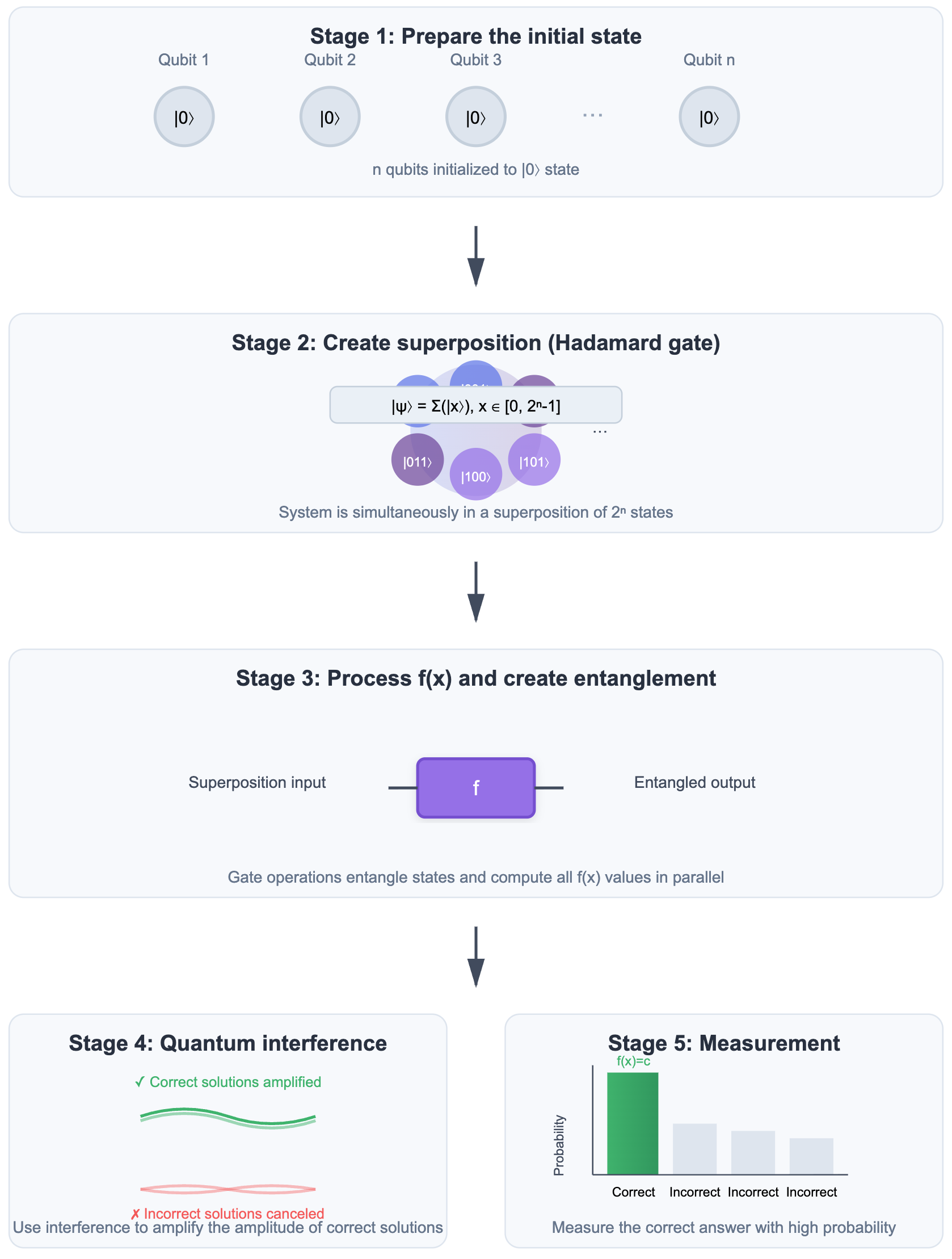
Figure: Core idea—superposition enables "parallelism"; making use of entanglement/interference to amplify the probability of correct solutions.

Note: Discussing quantum interference implicitly treats quantum states in wave form. If you’re curious why microscopic quantities admit wave descriptions, see Appendix 1.

Figure: Wave interference. Constructive interference boosts amplitude; destructive reduces it.

Of course, real quantum algorithms are far more complex than this intuitive description. Here we only provide a simplified explanation and do not involve specific algorithm details for now. If readers want to further understand why quantum algorithms pose a potential threat to classical cryptographic systems, please refer to Appendix 2.

Quantum Computing’s Acceleration Effects on Different Problems

The main sources of acceleration brought by quantum computers are:

Superposition states, meaning $n$ qubits can simultaneously represent $2^n$ states, equivalent to processing all possibilities in parallel at once.
Entanglement, through strong correlation between qubits, allows interference between different states, thereby effectively extracting useful information and amplifying correct answers.

This acceleration manifests differently for different types of problems. When suitable quantum algorithms are available:

Structured problems (such as integer factorization): Quantum algorithms can utilize their structure (such as periodic structure) to quickly extract answers through certain algorithms (such as quantum Fourier transform), thereby achieving exponential acceleration.
Unstructured problems (such as finding $x$ that satisfies $f(x)=c$): Due to the lack of patterns to exploit, we can only rely on continuous $\sqrt{N}$ times of interference to amplify the probability amplitude of the correct answer, so the number of computations can only be reduced from the classical $N$ times to $\sqrt{N}$ times, corresponding to square root level acceleration.

Part 2: How Are Quantum Computers Built?

Physical Implementations of Qubits

Qubits are essentially constructed from states in the physical world. Depending on the source of physical states used, quantum computer construction methods can be divided into two categories:

One approach uses microscopic particles—ions, photons, or atoms—computing by manipulating and measuring their quantum states. Identical particles have identical physical properties, enabling multi‑particle interference and entanglement. In well‑isolated settings, they offer high state purity, low error rates, and long coherence times. However, precise control remains challenging, and operations are typically slow.

Another approach uses artificial structures—such as superconducting circuits and quantum dots—where macroscopic circuit behavior encodes quantum states. These qubits are easier to fabricate, operate, and scale with modern semiconductor technology. The challenge is materials defects: unlike natural particles, each device has small variations that introduce noise and errors, reducing state stability. Even so, these qubits are generally easier to measure and control and are more tractable from an engineering standpoint.

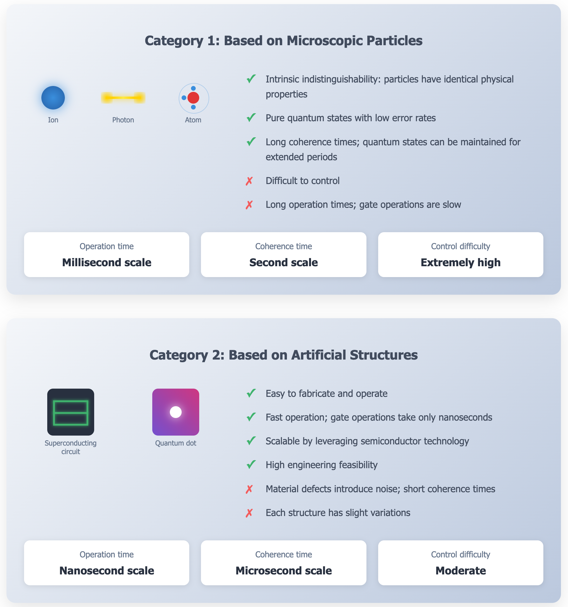
Figure: Two main approaches to building quantum computers.

Currently, superconducting quantum computing is considered one of the most mature and promising directions because it shows excellent performance in operating speed and integration, and its technological development is relatively rapid. Therefore, we will focus on introducing superconducting quantum computers as an example.

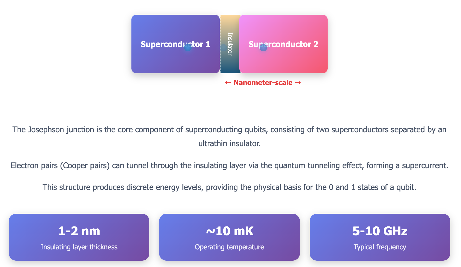
Construction Principles of Superconducting Qubits

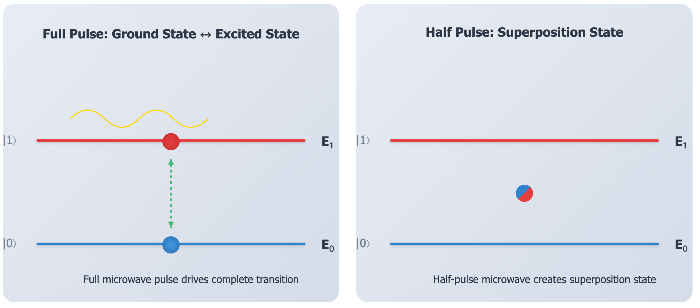
In superconducting quantum computers, the qubit state comes from the energy levels of a Josephson junction, the core device consisting of two superconductors separated by a nanometer‑scale insulator. Energy levels are the allowed energies of a system—discrete and fixed. The lowest level E₀ is the ground state; higher levels (such as E₁) are excited states. The qubit’s logical 0 and 1 correspond to E₀ and the first excited state E₁, respectively.

Figure: Josephson junction basic structure.

By applying microwaves at specific frequencies to the junction, we inject energy and drive transitions between E₀ and E₁ (much like a microwave oven drives molecular rotation with resonant microwaves). Precise control over these transitions underpins quantum logic. A “half pulse” can leave the qubit in a superposition of E₀ and E₁. In short, we steer qubit states by tuning the microwave frequency, amplitude, and duration.

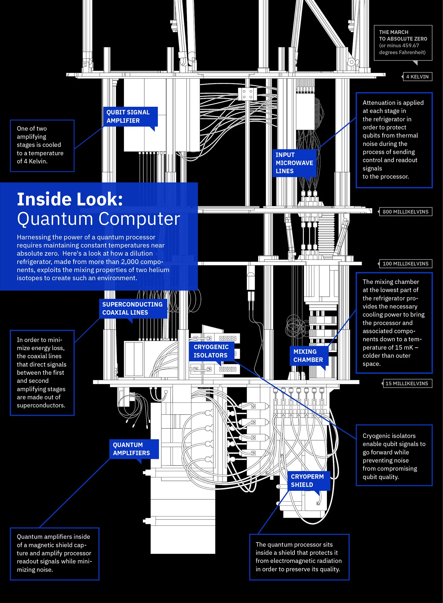
Figure: Energy‑level control of a superconducting qubit. A full pulse drives |0⟩→|1⟩; a half pulse creates a superposition.

Since the energy difference between the energy levels of superconducting qubits is extremely small, quantum states are extremely sensitive to disturbances from the external environment. Even very slight thermal noise, electromagnetic waves, or radiation interference can cause decoherence of quantum states (i.e., destruction of quantum states), preventing qubits from working properly. To reduce these interferences, superconducting quantum computers must operate in extremely low-temperature environments close to absolute zero (about 10 millikelvin (mK), only 0.01 degrees higher than absolute zero -273.15 °C, already the lowest continuous temperature humans can achieve), and use special materials and carefully designed shielding, filtering, and attenuation measures in connecting circuits to maintain energy level stability and manipulation precision as much as possible.

From Single Qubit to the “System Architecture” of Superconducting Quantum Computing

To build a practically operational superconducting quantum computer, not only qubits themselves are needed, but also a complete support system: refrigeration and shielding systems to protect quantum states, control systems to manipulate qubits, and error correction systems to correct errors in quantum systems in real time. Among these systems, the error correction system is particularly critical. This is because the reliability of quantum computing faces two fundamental challenges:

Insufficient coherence time: That is, the duration a qubit can maintain quantum properties such as superposition and entanglement without being destroyed by the environment. Therefore, to use qubits for computation, the coherence time of qubits must be longer than the time required for computation. Although measures such as refrigeration and shielding can extend coherence time, they are still difficult to meet the demands of complex operations.
Insufficient gate fidelity: Quantum gates are not fixed gate circuits like classical bits, but are implemented through real-time manipulation by external control signals. The closeness of the actual effect of quantum gate operations to the ideal effect is the gate fidelity. However, even if the fidelity of a single gate operation is very high (such as 99.9%), after performing thousands or even millions of operations, errors will continue to accumulate, ultimately destroying computational results.

Next, we will introduce each core component of superconducting quantum computers in detail:

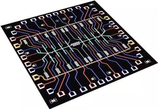
Quantum Chip

Josephson junctions are fabricated on silicon using conventional semiconductor processes to form qubits, and the package brings out control and readout interfaces.

Figure: Quantum chip (processor) with 20 superconducting qubits. Each qubit has control/readout lines; couplers provide switchable interactions.

Refrigeration System

A dilution refrigerator (using a helium‑3/helium‑4 mixture) cools the quantum chip and wiring to near absolute zero—down to ~10 mK or below. Along the signal path, attenuators and filters condition control signals, and shielding reduces external noise to preserve fragile quantum states.

Figure: IBM Q refrigeration stack inside a dilution refrigerator. Coaxial lines handle control/readout; inputs pass through multi‑stage attenuators; outputs use low‑noise amplifiers. Multi‑layer shields block radiation. Temperature steps from room temperature to ~10 mK to stabilize qubits.

Qubit Control System

Converting quantum operation instructions issued by classical computers into high‑precision microwave pulses for driving, manipulating, and reading qubits, typically including devices such as microwave generators, mixers, amplifiers, and isolators.

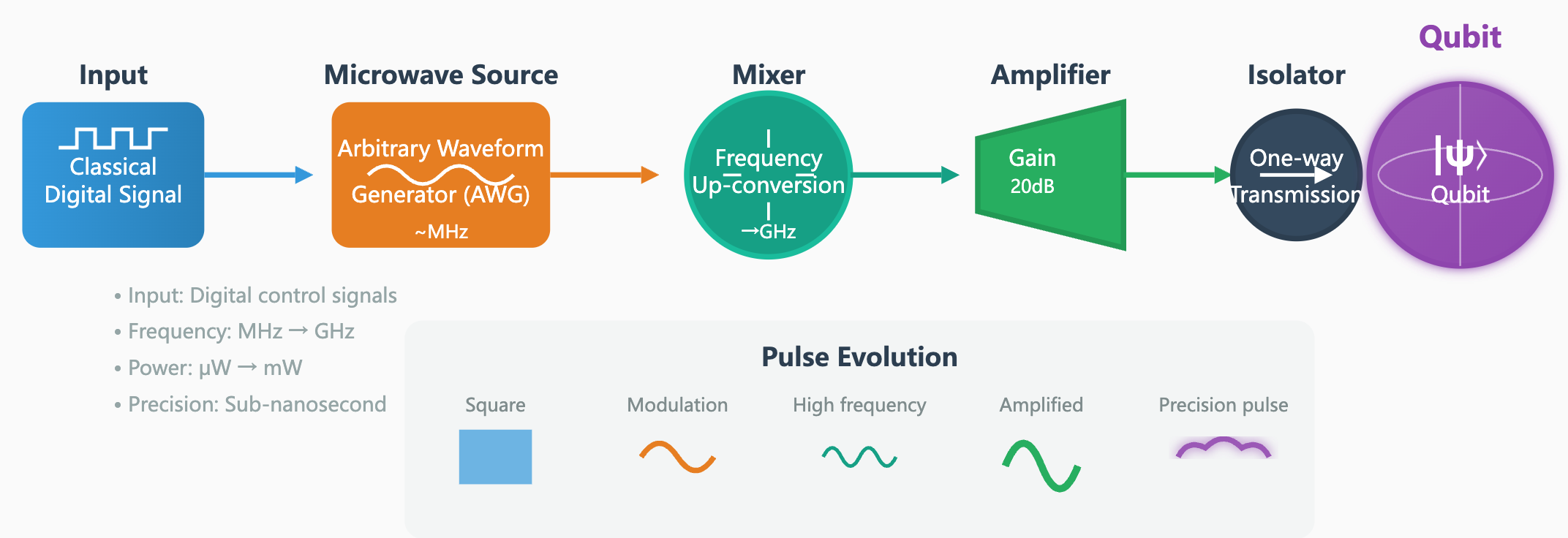
Figure: Qubit control system. Digital commands become precise microwave pulses with high purity and tight timing for accurate state control.

Quantum Error Correction System

Through redundant encoding and real‑time feedback, the system detects and corrects errors caused by decoherence and noise, extending coherence time and improving gate fidelity. For example, the widely used surface code encodes a logical qubit into a two‑dimensional array of qubits and repeatedly measures correlations between neighbors to find and correct errors, prolonging logical‑qubit lifetime when hardware error rates are below threshold.

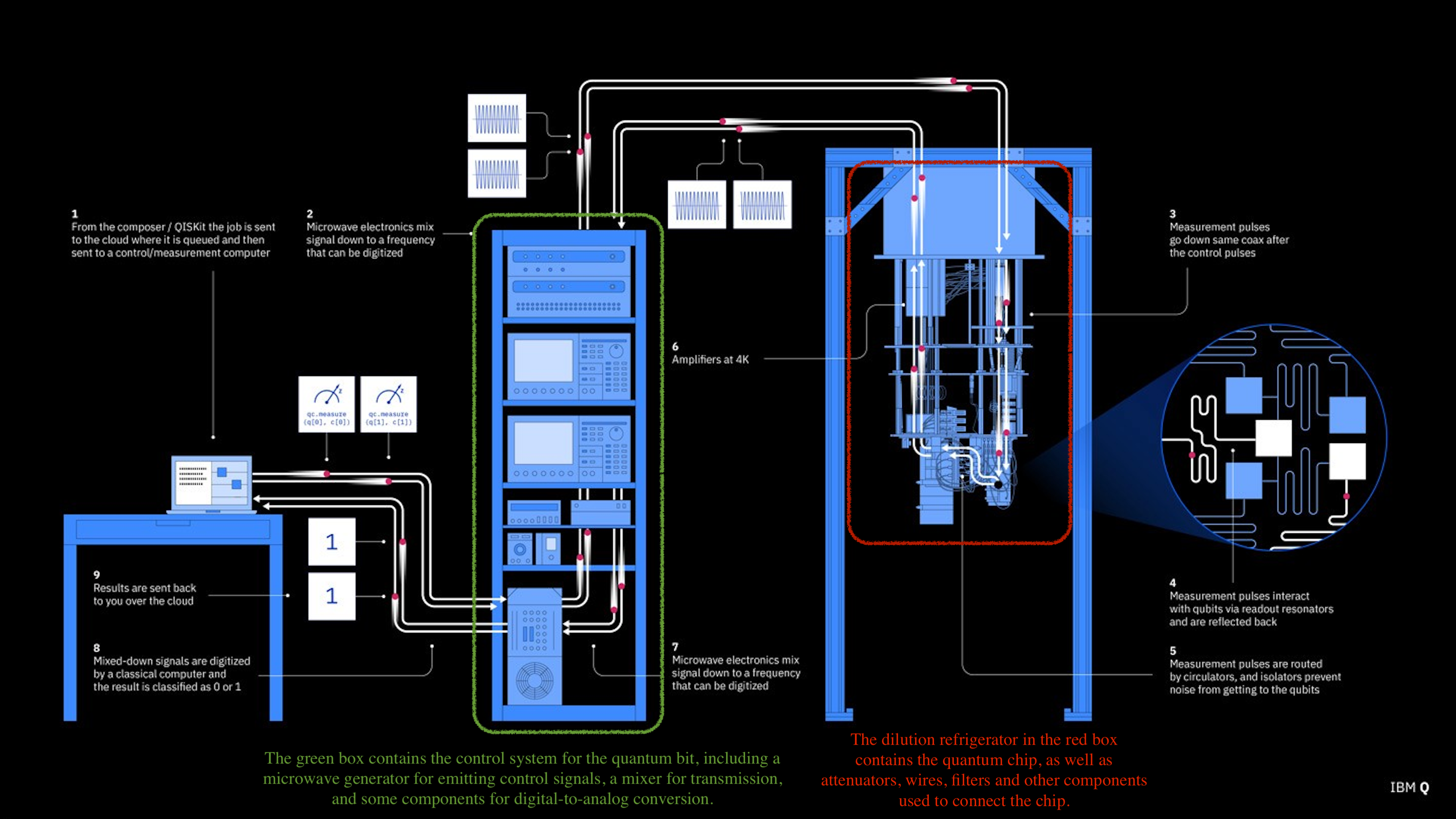
Figure: Quantum error correction loop must run well within coherence time. Low‑latency FPGA plus CPU/GPU compute and tight timing enable real‑time correction.

Overall Architecture

The figure below shows the overall architecture of a quantum computer.

Figure: IBM Q system architecture. Components described above are shown in the figure.

Building Quantum Computers Requires Combining Science and Engineering

The construction of quantum computers is both physics and engineering. Particle-based solutions are purer at the physical level but difficult to implement in engineering; artificial structure-based solutions (especially superconducting qubits) are more scalable in engineering but need to overcome noise and decoherence problems. A complete superconducting quantum computer is essentially a complex combination of quantum chip + dilution refrigerator + control electronics + quantum error correction system. It is both a physical experimental device and a highly engineered system. It is precisely because of this “from physics to system” complete chain that superconducting quantum computers have become the most promising solution to cross the practical threshold first.

Part 3: What Challenges Remain in Building a Quantum Computer Capable of Breaking RSA 2048?

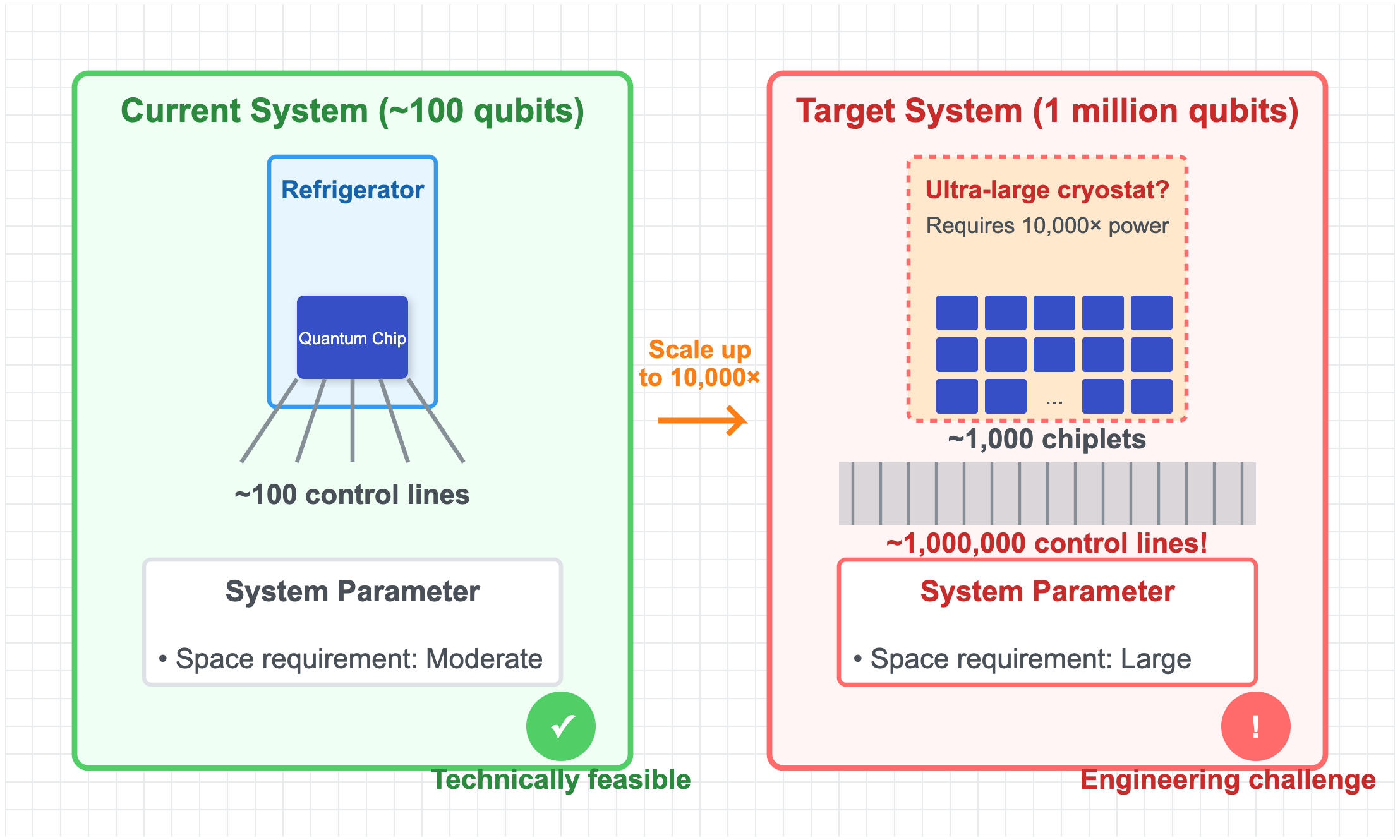
Today’s more mature superconducting quantum computers typically have on the order of hundreds of qubits. As noted in Part 1, quantum computers can accelerate integer factorization. Shor’s algorithm requires roughly 2N qubits to factor an N‑bit integer, plus ancilla registers and other overhead. To break RSA‑2048, the total would be on the order of several thousand qubits.

That might sound close to success—but not quite. To complete the computation, qubit coherence time must exceed the time needed for all required operations. Today, superconducting‑qubit coherence times are usually tens to hundreds of microseconds, while gate times are tens to hundreds of nanoseconds. Shor’s algorithm requires on the order of 10¹² quantum‑gate operations, far exceeding typical coherence times. Even if we could finish within coherence time, gate fidelity would still limit performance: at 99.9% per gate, tiny errors accumulate over 10¹² operations and ruin the result.

Therefore, we must rely on quantum error correction to break through these physical bottlenecks. Taking surface code as an example, by encoding a large number of physical qubits into one logical qubit, it effectively extends “usable coherence time” and offsets cumulative errors in gate operations. Based on current error rates and error correction schemes, one logical qubit typically requires thousands of physical qubits. In other words, to obtain thousands of logical qubits to run Shor’s algorithm, the total number of physical qubits actually required will reach the million level.

Next, we will introduce in detail the technical obstacles that each core component of quantum computers needs to cross to expand the number of superconducting qubits from hundreds to millions.

Quantum Chip

The quantum chip—where qubits (Josephson junctions) reside—is also called a quantum processor. Scaling to more qubits faces three main difficulties: wiring, crosstalk, and semiconductor yield.

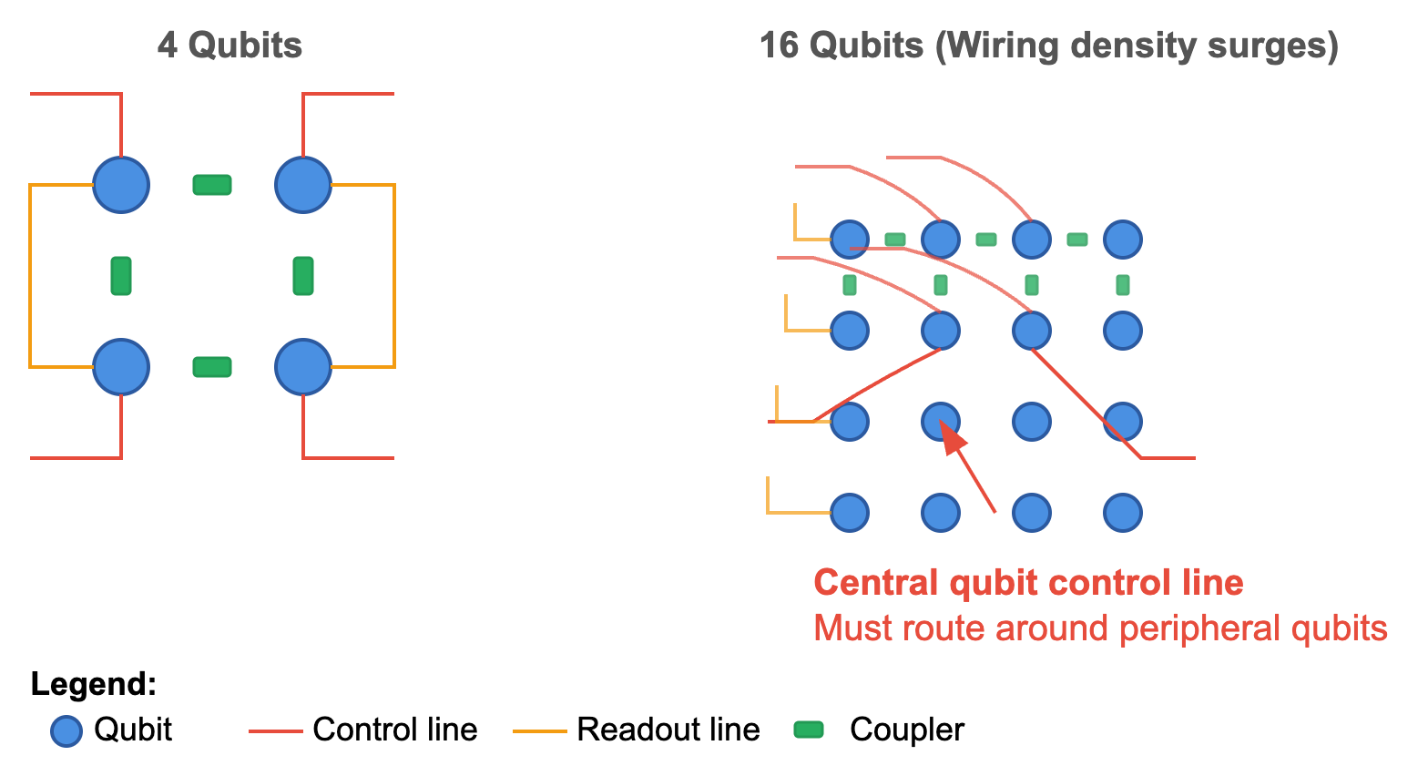
Wiring Problem

Each qubit requires multiple lines (control and readout), and couplers interconnect qubits. On a two‑dimensional chip, as qubit count rises, wiring complexity grows nonlinearly. In highly connected layouts, control lines for central qubits must snake around peripheral ones, dramatically increasing chip area.

Figure: Wiring complexity grows nonlinearly with qubit count.

Crosstalk Problem

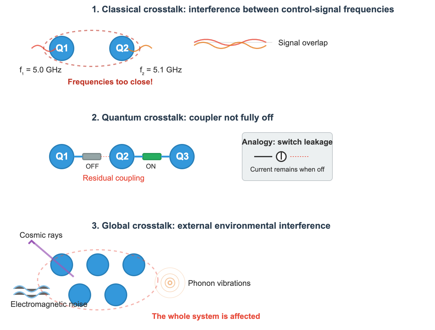
Crosstalk—mutual interference between qubits—causes decoherence and grows nonlinearly with system size. Common forms include:

Classical crosstalk: control frequencies are too close, causing unintentional drive. (In quantum processors, each qubit is driven at a specific microwave frequency.)
Quantum crosstalk: residual coupling that fails to turn fully off (analogous to current leaking through an “open” classical switch).
Global crosstalk: interference from external physical processes such as cosmic rays or phonons.

To mitigate crosstalk, designers may add isolation regions and shielding, and improve coupler devices to achieve better off‑state isolation. Enhancing the control/readout stack—especially frequency planning—also helps reduce crosstalk during parallel two‑qubit gates.

Figure: Crosstalk grows nonlinearly with qubit count and harms coherence.

Device Yield Problem

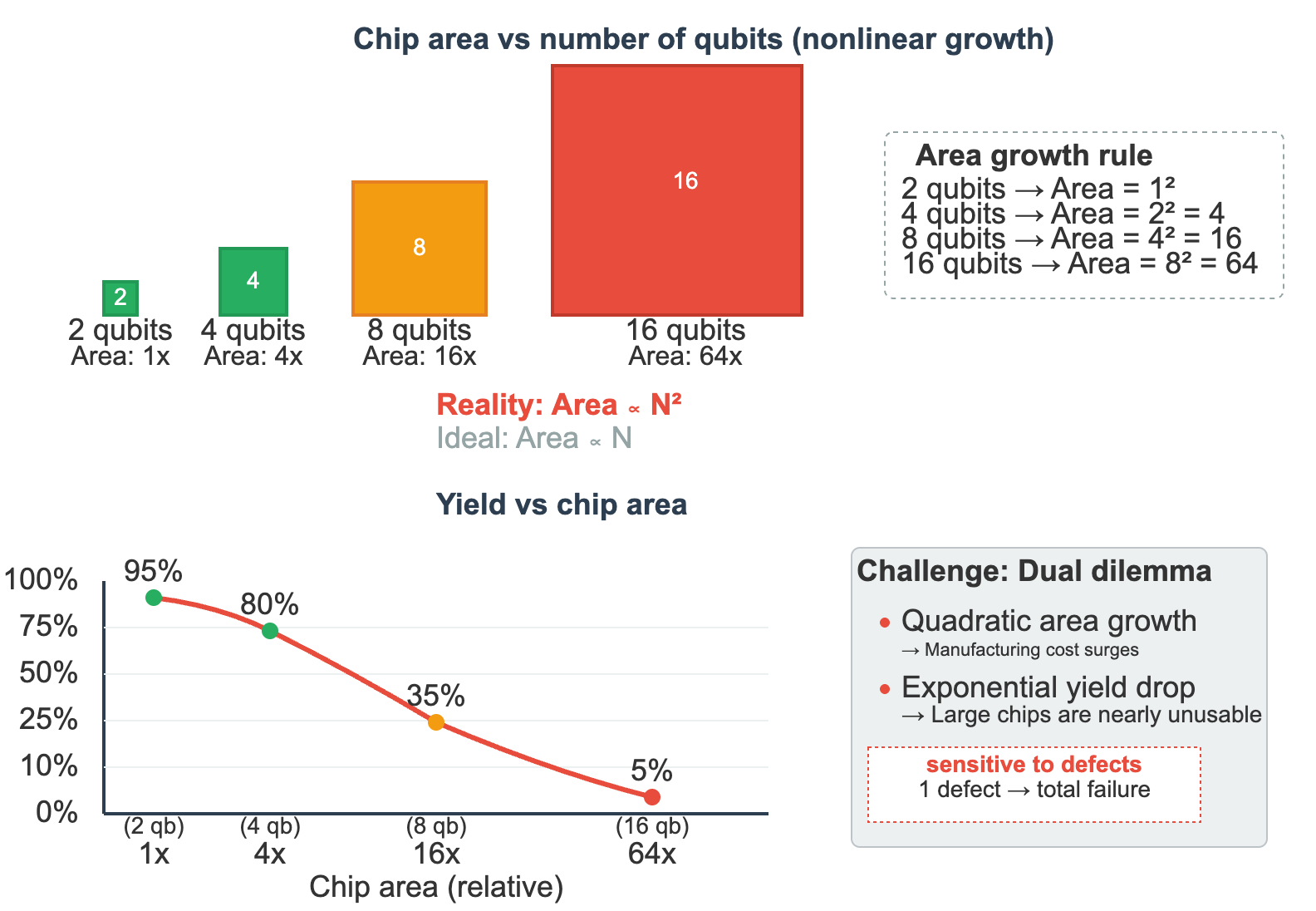
If looking only at area, the area of quantum chips should be linearly related to the number of qubits. However, due to the need to handle wiring and crosstalk problems, actual chip area often approaches square growth with the number of qubits. In other words, the more qubits, the more nonlinearly the chip area expands.

More troublesome is that quantum bits are extremely sensitive to defects, and even a 1% failure rate will make the entire system unusable. If there are defects inside or on the surface of the chip, they may couple with quantum bits, reducing their coherence time. In the field of micro-nano processing, there is a basic rule: the larger the chip area, the lower the yield, and the manufacturing difficulty of large-area chips increases exponentially. For superconducting quantum chips, although their manufacturing process can borrow mature equipment and process flows from the semiconductor industry, the extreme sensitivity of quantum bits to manufacturing defects makes the yield problem a huge challenge.

Figure: Area scales ~N² as qubit count grows; yield typically falls with die area (illustrative values).

Hope on the Horizon: Modular Design and Inter-Chip Interconnection

Wiring, crosstalk, and yield all worsen nonlinearly with scale. Building a million qubits on a single chip is therefore unrealistic.

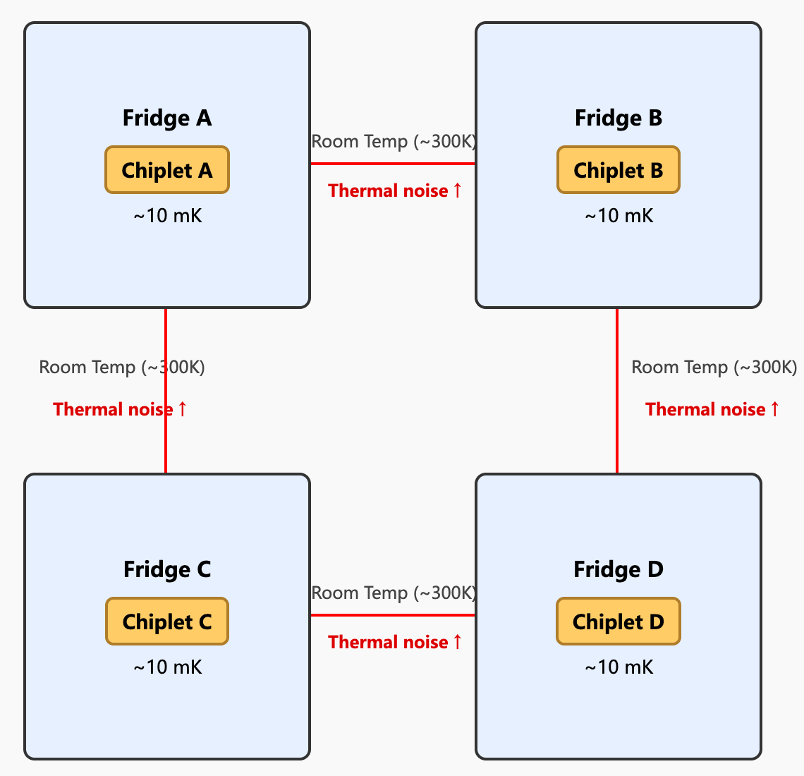
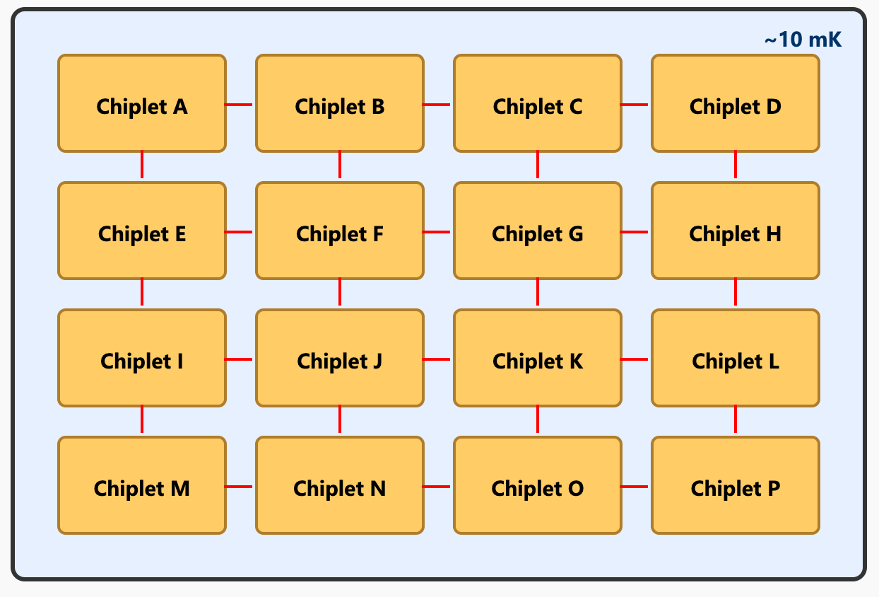
A more feasible path is modular: first build chiplets with thousands of physical qubits (enough to form reliable logical qubits), then connect them with inter‑chip interconnects. This reduces the single‑die challenge from “hundreds to millions” down to “hundreds to thousands.”

However, this idea also brings new problems. Quantum bits are very fragile and must work in low-temperature environments around 10 millikelvin. If each chiplet is placed in an independent dilution refrigerator, then to achieve interconnection between chiplets, signal lines would need to be led out from the low-temperature environment of one refrigerator to room temperature, then enter the low-temperature environment of another refrigerator.

This “low temperature ↔ room temperature ↔ low temperature” signal transmission path will introduce large thermal loads and noise, thereby destroying the state of qubits. If all chiplets are placed in the same dilution refrigerator, then we need an extremely powerful dilution refrigerator to accommodate thousands of chiplets, and manufacturing such a large‑scale dilution refrigerator is itself a new challenge.

Figure: Chiplet links across separate refrigerators introduce thermal noise. Topology shown is illustrative.

Figure: Multiple chiplets in a single refrigerator with direct low‑temperature links. This centralized design needs ultra‑high‑power refrigeration. Topology shown is illustrative.

Going forward, either cross‑refrigerator links must suppress added noise, or dilution refrigerators must scale dramatically. Given today’s science and engineering, the latter—higher‑power, larger‑volume dilution refrigerators—appears more achievable.

Summary

If we adopt chiplets plus inter‑chip interconnects, the chip‑level challenge is expanding a single die from hundreds to thousands of qubits.

The good news: semiconductor manufacturing is a well‑developed technology stack, and related processes continue to improve. For example, advanced‑packaging 3D stacking can boost wiring density and interconnect capability. Better superconducting materials and processes, multiplexed designs, and smarter chip architectures (e.g., higher‑isolation couplers, more effective frequency planning) will also help.

Thus, expanding a single chip from hundreds to thousands of physical qubits, while challenging, is primarily an engineering bottleneck and looks relatively tractable. Currently, IBM has demonstrated a single chip with 1,000 physical qubits; large die size, however, raises yield and within‑chip reliability concerns for mass production.

Refrigeration System

Since the energy level difference of superconducting qubits is very small, quantum states are extremely susceptible to disturbances from the external environment and decohere. Currently known main interference factors include:

Passive thermal sources: Although qubits are in an environment close to absolute zero, they must be connected to room‑temperature electronic equipment through wires. Wires act like a “thermal bridge,” bringing heat from high‑temperature environments to low‑temperature areas.
Active thermal sources: Manipulating qubits requires sending microwave pulses, which are transmitted along wires. During transmission and attenuation, energy always converts to heat, which accumulates and heats the environment.
Thermal radiation: Even if wires and materials are isolated, there is still electromagnetic radiation coupling between quantum chips and the outside world. High-temperature environments will “radiate heat” to low-temperature chips.

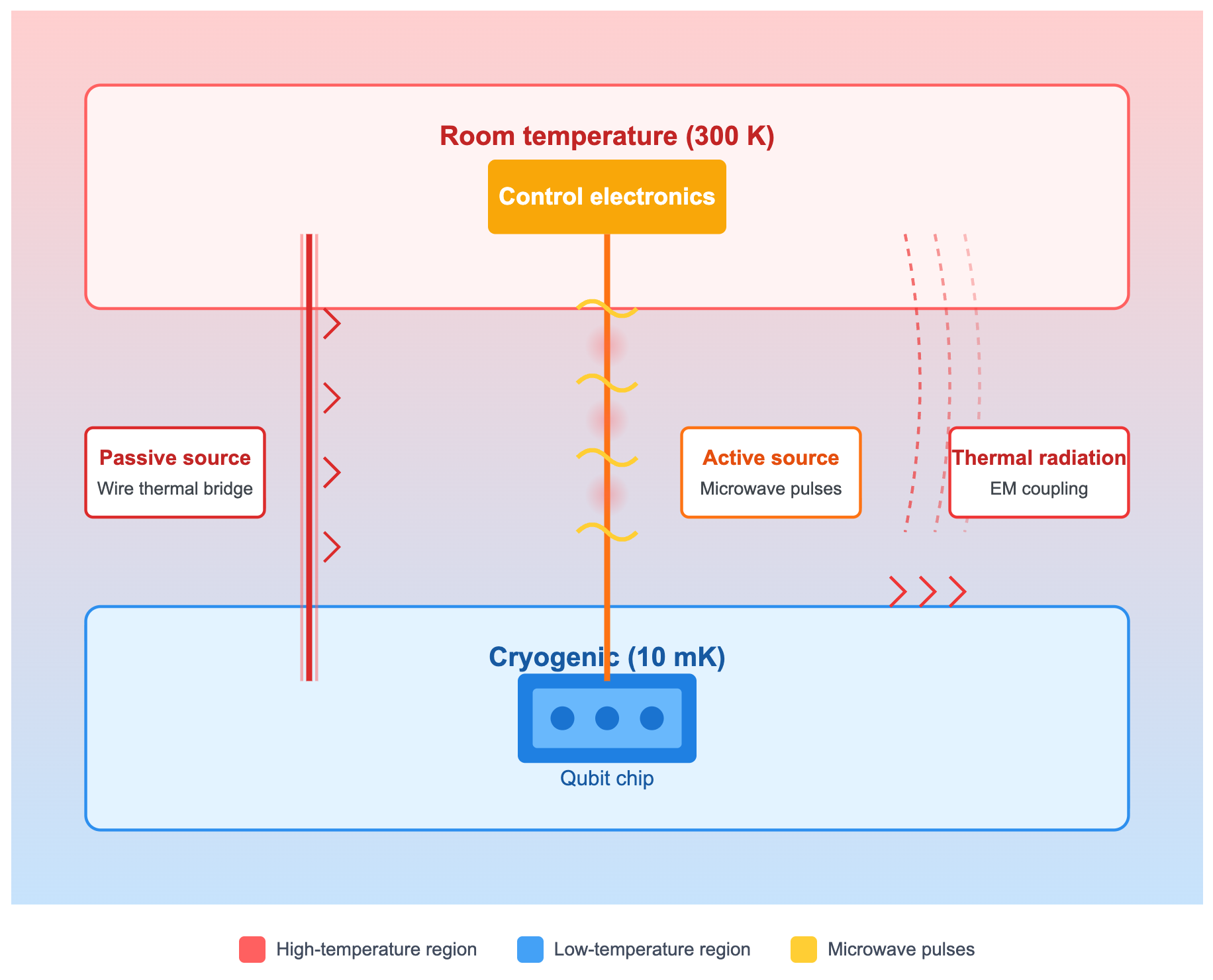
Figure: Three main thermal interference sources for qubits.

To isolate these effects as much as possible, current practice is:

Use materials with appropriate thermal and electrical conductivity to make wires;
Add filters and attenuators in signal paths to weaken unnecessary frequency bands and dissipated energy from control signal transmission;
Use dilution refrigerators for staged cooling (not directly cooling from room temperature to 10 mK, but sequentially through room temperature → 50 K → 4 K → 1 K → 100 mK → 10 mK), progressively shielding thermal sources.

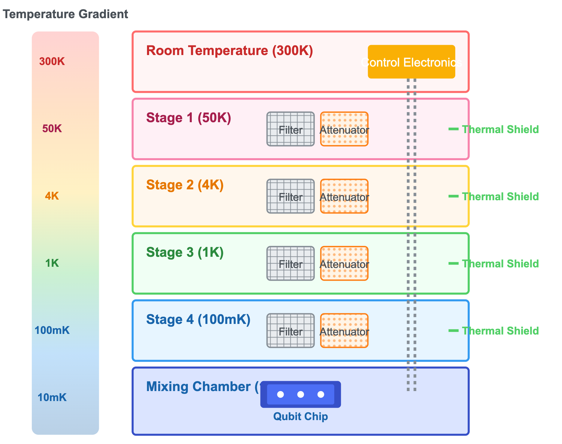
Figure: Staged cooling in a dilution refrigerator: thermal buffers isolate heat, filters remove unwanted bands, attenuators absorb excess energy, and shields block radiation.

This approach currently supports systems with on the order of hundreds of physical qubits. To reach millions (e.g., thousands of chiplets with thousands of qubits each), a scaling problem emerges: each qubit needs wires, attenuators, and filters, and these scale roughly linearly with qubit count. While a single wire’s thermal leak is small, a million such components overwhelm cooling capacity. Beyond more powerful refrigerators, we need aggressive multiplexing, cryogenic CMOS (cryo‑CMOS), and low‑temperature superconducting electronics to cut wiring and power.

In short, the cooling power and physical space of existing dilution refrigerators are seriously insufficient. To support a million-bit system, the refrigerator’s power needs to increase by at least a million times or more. But such ultra-high-power, ultra-large-volume dilution refrigerators do not yet exist.

Figure: Refrigeration must scale from hundreds to millions of qubits.

If adopting a “chiplet design” + “low‑temperature inter‑chip interconnect” scheme, then the refrigeration system is a major engineering hurdle that must be crossed, requiring enormous R&D investment (likely in the tens of billions of dollars range).

Qubit Control System

As noted earlier, each superconducting qubit is controlled with microwaves, and different qubits are assigned different drive frequencies. Scaling from hundreds to millions raises several challenges:

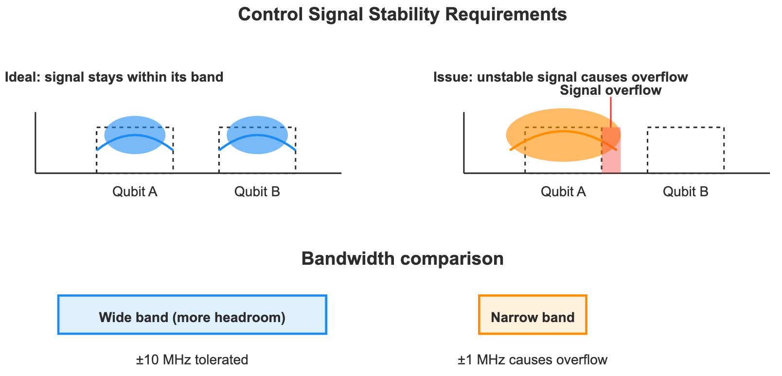
Frequency crowding: The microwave spectrum range is limited. As the number of bits increases, frequency intervals are forced to decrease. When adjacent frequencies are too close, control signals may interfere with each other, causing crosstalk problems.

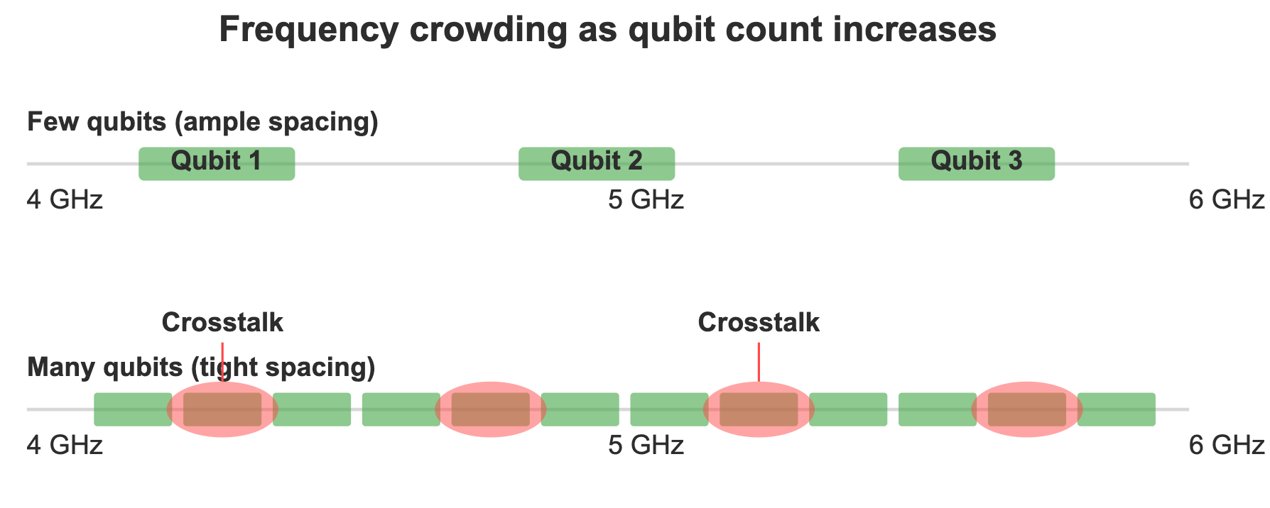
Figure: Adjacent drive frequencies can interfere, causing crosstalk.

Increased precision requirements: Narrower frequency bands mean control signals must be more stable, otherwise they will “overflow” to adjacent bits. Requirements for frequency stability and phase noise become more stringent.

Figure: Narrower bands demand better frequency stability and lower phase noise; small drifts can spill into adjacent qubits.

Soaring control complexity: Each qubit requires independent pulse control (amplitude, phase, timing). If there are a million qubits, there must be a million independent control channels. Currently, the hardware cost per channel is approximately ¥100,000/channel, with the long‑term goal of reducing it to ¥1,000/channel, otherwise the cost will be unbearable.

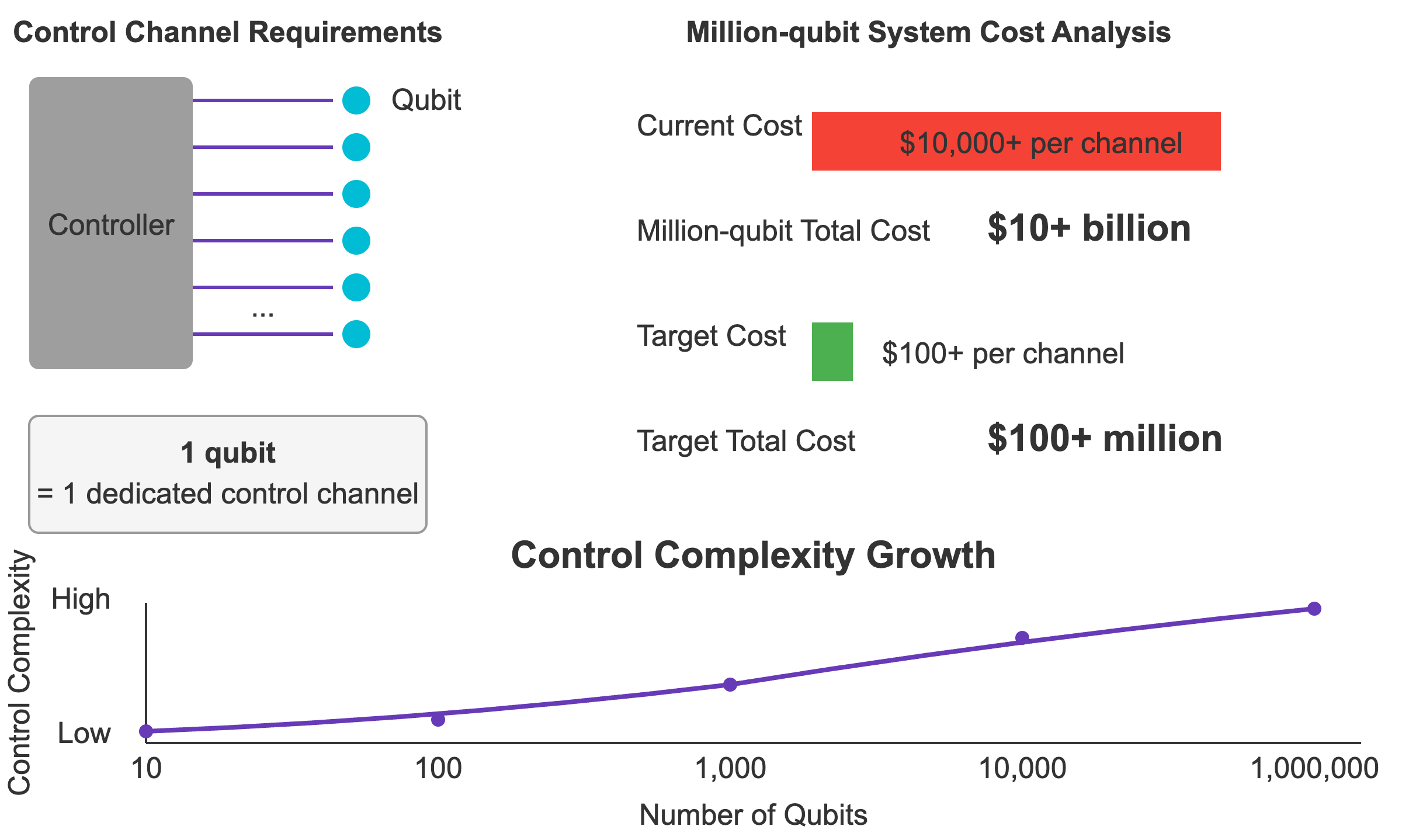
Figure: A million qubits require a million independent control channels.

These problems are essentially engineering bottlenecks. They have already appeared in small‑scale systems, and complexity increases linearly as scale expands.

However, the challenges in this direction are generally considered relatively optimistic compared to other issues in the industry, mainly for the following reasons:

Pattern of frequency crowding: Experiments show that within a few dozen qubits (≈60), frequency planning becomes rapidly more complex, but with more qubits, frequency reuse and careful layout can keep complexity manageable. So “frequency crowding” is not necessarily a hard barrier.
Limited gate precision requirements: Quantum computing does not require infinite precision. As long as two‑qubit gate fidelity can stabilize around 99.99%, it is sufficient to support quantum error correction. Although this still requires very high noise control for the control system, it is achievable with existing semiconductor technology. The only issue is that high‑speed digital‑to‑analog converters (DACs) capable of achieving this precision are currently too expensive. Whether costs can be reduced through large‑scale manufacturing remains to be seen.
Potential for hardware cost optimization: Current control stacks rely on superconducting coaxial cables, adapters, attenuators, and filters—expensive and bulky. Borrowing flexible‑substrate processes from semiconductors to mass‑produce integrated cryogenic wiring on low‑cost materials could cut both cost and volume.

In summary, the control system is another engineering bottleneck that must be crossed: million‑qubit systems require a million independent control channels, with frequency allocation, signal precision, and cost reduction all being key difficulties. Although relatively more optimistic compared to other issues, it still requires long‑term engineering investment and technological iteration.

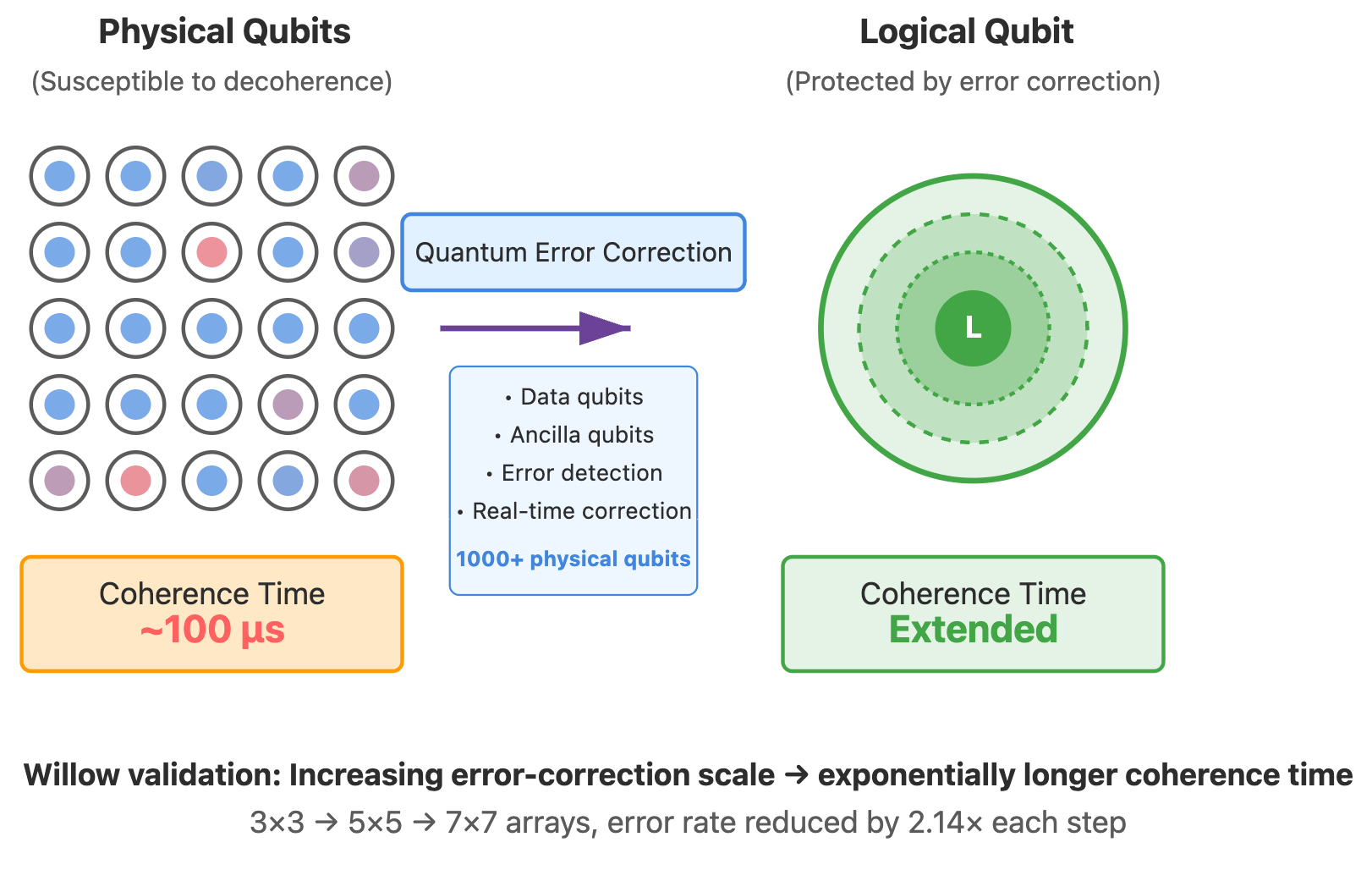
Error Correction System

To make qubit and gate fidelity meet the requirements for completing large‑scale computations like factoring RSA, we must rely on quantum error correction (QEC): using thousands of physical qubits to form one logical qubit.

The theoretical framework of quantum error correction is mature and can significantly improve coherence time and gate fidelity of logical qubits. For example, Google’s Willow project demonstrated more stable logical qubits through error correction.

In the Willow processor, a logical qubit is not directly represented by a single physical qubit but is jointly encoded by a two‑dimensional physical‑qubit array. The array contains two types of qubits:

Data qubits: Used to carry logical quantum states;
Ancilla qubits: Through periodic operations to detect whether errors have occurred between data qubits.

The measurement results of these ancilla qubits do not directly reveal the logical state itself but can reflect whether errors such as bit flips or phase flips have occurred in the system. Combined with decoding algorithms, the system can determine where errors occurred and make corrections. In Willow’s experiments, researchers verified this key characteristic on hardware for the first time: when the physical‑qubit error rate drops below the threshold, theoretically, as long as engineering allows, the effective coherence time of logical qubits can be continuously extended by increasing encoding scale, and the fidelity of logical gates can be continuously improved. In other words, the ultimate limitations on coherence time and gate fidelity mainly come from engineering resources, not fundamental physical laws.

Figure: Many noisy physical qubits can encode a stable logical qubit; larger codes extend coherence as needed.

However, in engineering implementation, decoding algorithms must be real-time: if errors accumulate too quickly, they will exceed the recoverable range. As the number of bits increases, error correction overhead grows nonlinearly, imposing extremely high requirements on classical hardware computing power and latency. Fortunately, error correction computation itself can be highly parallel, so theoretically bottlenecks can be alleviated by increasing computing power (i.e., “throwing money at it”).

The challenge is not only at the physical level but also in software‑hardware integrated engineering: since qubits continuously generate random errors that cannot be known before operation, circuits must dynamically adjust subsequent operations based on error information detected on‑site. At the same time, the error correction system must also implement real‑time scheduling and calibration of logical qubits and complete parallel decoding under extremely low latency. These requirements stacked together make fault‑tolerant quantum computing not only a hardware challenge but also a system engineering project of enormous scale and extremely high complexity.

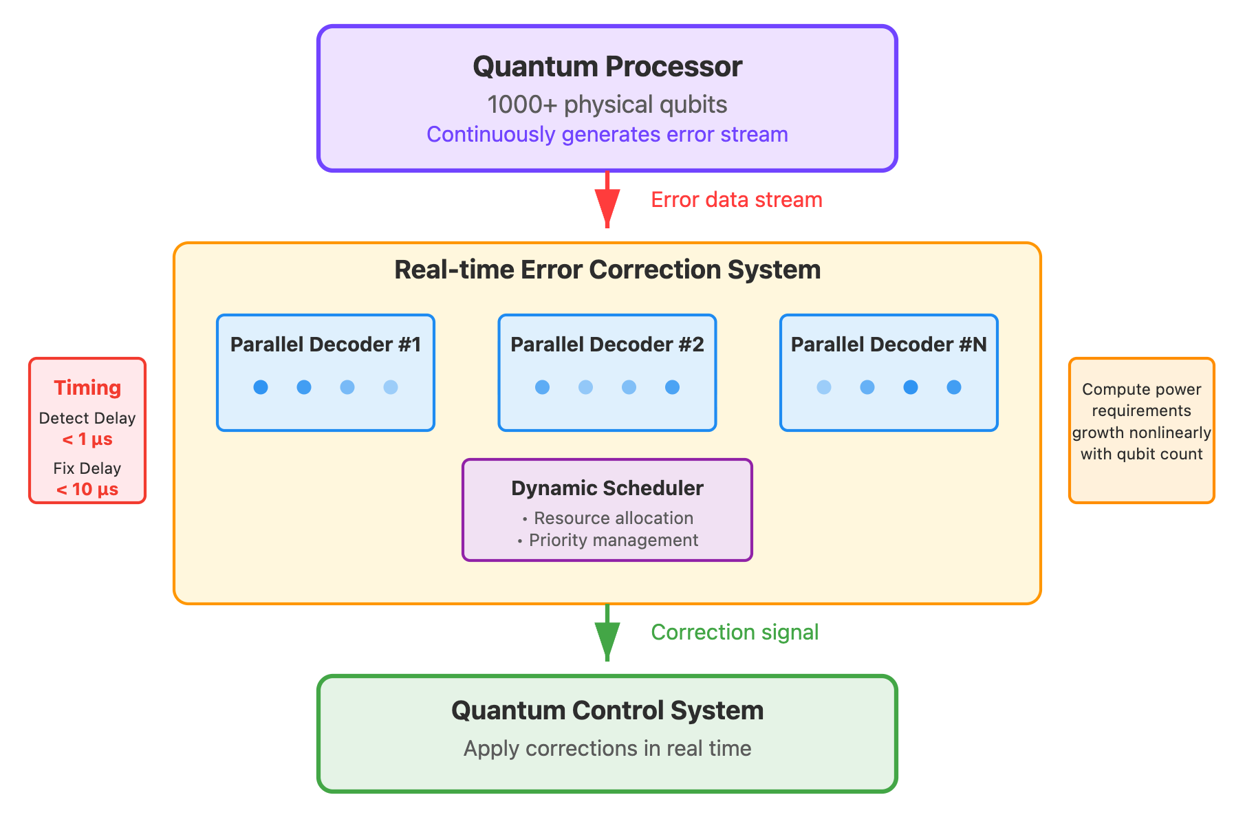
Figure: QEC is a demanding systems problem: detect errors, decode in parallel, and correct within microseconds; compute demands grow with scale.

In summary, the quantum error correction system is a threshold that must be crossed: it requires thousands of physical qubits to form one logical qubit and relies on real‑time, parallel error correction and dynamic scheduling, imposing extremely high requirements on software‑hardware integration and representing an extremely challenging system engineering project. However, the entire process has no scientific limitations that cannot be solved—it is more a challenge of system engineering.

Quantum Computers Capable of Breaking RSA-2048 Will Likely Appear in the 2030s

In summary, to manufacture a million‑qubit computer capable of breaking RSA‑2048, the scientific challenge lies in the unavoidability of decoherence and gate errors, but quantum error correction theory has provided a clear solution path; the real difficulty is at the engineering level, including cooling, control, wiring, energy consumption, and real‑time implementation of quantum error correction. As scale expands, these problems will show nonlinear amplification, especially crosstalk, error correction overhead, and energy consumption. However, after a certain scale, modular design and inter‑chip interconnection can make complexity enter a regionally linear phase. Overall, there are no scientific “dead ends,” but engineering challenges are extremely large, requiring long‑term accumulation and huge investment. Currently, the industry generally expects such quantum computers to appear in the 2030s with high probability, and we agree with this judgment.

Appendix 1: Mathematical Expression of Superposition States and Entanglement

Vector Expression of Superposition States and Collapse

In quantum mechanics, for a single quantum state, we can express it in vector form:

$$ |\psi\rangle = \alpha |S_0\rangle + \beta |S_1\rangle $$

Where:

$|S_0\rangle$ and $|S_1\rangle$ are two possible states of the quantum system;
$\alpha$ and $\beta$ are called complex probability amplitudes, whose modulus squared gives the probability of obtaining the corresponding state during measurement, and they satisfy $|\alpha|^2+|\beta|^2=1$.

Quantum computers select two distinguishable physical quantum states from a physical system as information carriers, denoted as $|0\rangle$ and $|1\rangle$, respectively. Therefore, the state of a quantum bit (qubit) can be written as:

$$ |\psi\rangle = \alpha |0\rangle + \beta |1\rangle $$

Vector Expression of Quantum Entanglement

If two qubits are prepared in an entangled state where they must have different values (an odd‑parity Bell state), then the system’s state is:

$$ |\psi\rangle = \alpha |01\rangle + \beta |10\rangle $$

Where $\alpha$ and $\beta$ are complex probability amplitudes satisfying the normalization condition $|\alpha|^2+|\beta|^2=1$.

This means: the probability of measurement result “01” is $|\alpha|^2$, the probability of measurement result “10” is $|\beta|^2$, while the probabilities of “00” and “11” are strictly zero. It can be seen that quantum entanglement is actually an extension of superposition states in multi-dimensional bases.

Wave Function Expression of Quantum States

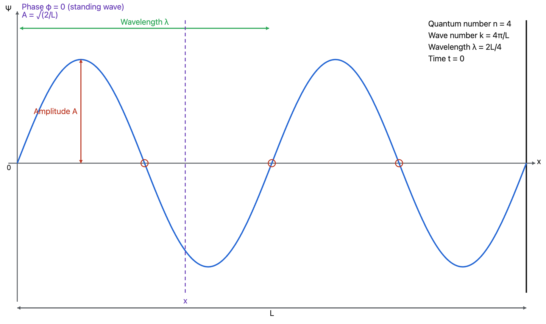
Quantum states can also be described in wave form, with the modulus square of the wave function giving the probability of collapsing to a specific state. Taking a particle confined in a one-dimensional box (with impassable walls at both ends) as an example, the particle’s waves reflect at both ends and superpose on each other (similar to sound echoing between two walls), and the wave function manifests as a standing wave.

$$ \psi_n(x,t) = \sqrt{\frac{2}{L}} \sin\left(\frac{n\pi x}{L}\right) e^{-i\omega_n t} $$

Where $t$ is time, $x$ is the particle’s position, $L$ is the box length (range of particle motion), $n$ is the quantum number (1,2,3…, determining how many peaks and troughs the wave function has), $k = \frac{n\pi}{L}$ is the wave number (i.e., spatial frequency), $\lambda = \frac{2\pi}{k} = \frac{2L}{n}$ is the wavelength (i.e., spatial period), $\omega$ is the angular frequency, and the wave’s temporal frequency $f = \frac{\omega}{2\pi}$. The probability of the particle appearing at position $x$ at time $t$ is $|\psi(x,t)|^2$. The passage of time only adds a string of rotating phase factors to the entire wave function, not affecting the probability distribution.

Figure: Wave function (real part) at t=0.

Relationship Between Wave Function Expression and Vector Expression of Quantum States

Some readers might wonder: the state‑vector form $|\psi\rangle = \alpha |S_0\rangle + \beta |S_1\rangle$ and the wave‑function form $\psi_n(x,t)$ seem unrelated. In fact, they are two representations of the same quantum state in different “coordinate systems.”

To describe a quantum state at a certain moment (assume $t=0$), we must first choose a set of bases.

The first method uses continuous position basis ${|x\rangle}_{0<x<L}$. In this case, the abstract quantum state can be described as $\psi(x)=\langle x | \psi \rangle$, called the wave function, which assigns a complex amplitude to each point $x$.
The second method uses discrete energy basis ${|n\rangle}$. In this case, the abstract quantum state can be described as $|\psi\rangle = \sum_n c_n|n\rangle$, where $c_n=\langle n|\psi\rangle$, which assigns a complex amplitude to each energy eigenstate.

These two representations are related by:

$$ \psi(x)=\sum_n c_n\sqrt{\frac{2}{L}}\sin(\frac{n\pi x}{L}) $$

These two notations are just different perspectives; they essentially describe the same physical quantity.

Appendix 2: How Quantum Algorithms Threaten Classical Cryptography

To make it understandable for readers unfamiliar with mathematics or physics, this section will minimize the use of complex mathematical formulas. This may result in some inaccuracies in details but will not affect overall understanding.

Grover’s Algorithm: Accelerating Search Problems

Bottleneck of Classical Search

Suppose you have a black-box function $f(x)$ that can determine whether a certain input $x$ is the correct answer:

$f(x) = 1$: indicates $x$ is the target
$f(x) = 0$: indicates $x$ is not the target

If $x$ is a 32-bit integer, there are $2^{32}$ possible values. On a classical computer, we can only try $f(x)$ one by one, requiring $2^{32}$ tries in the worst case.

How Does Quantum Computing Accelerate Search?

Quantum computers reduce search complexity from $O(N)$ to $O(\sqrt{N})$ through superposition states and interference. The core logic of Grover’s algorithm is as follows:

Construct superposition state. Quantum computers can make variable x simultaneously represent a superposition state of all possible values, that is, $x = 0, 1, 2, \cdots, 2^{32} - 1$. If these values are substituted into $f(x)$, then $f(x)$’s result will also be a superposition state of all possible outputs. For some $x$, $f(x)$’s value is 0; for other $x$, $f(x)$’s value is 1.
Mark the correct answer (Oracle operation). The key to Grover’s algorithm is “marking the correct answer.” In quantum computing, this marking does not directly tell you the answer but makes the correct answer special at the quantum mechanical level through operations. For example, we do special processing on those $x$ where $f(x) = 1$ (i.e., correct answers): change their “phase.” Phase is a property of quantum states that, while invisible itself, can affect the probability distribution when quantum states collapse through subsequent operations. This step is equivalent to putting an “invisible mark” on the correct answer.
Amplify the probability of the correct answer through interference. Next, through constructive interference, the amplitude of the correct answer is gradually amplified, and through destructive interference, the amplitude of wrong answers is gradually reduced. This can be imagined as an “amplifier”—each operation makes the presence of the correct answer stronger. Each interference operation further increases the probability of the correct answer. After approximately $\sqrt{N}$ Oracle operations, the probability of the correct answer approaches 1.
Measure the correct answer. Finally, by measuring the quantum state, the quantum computer can almost always return the correct answer.

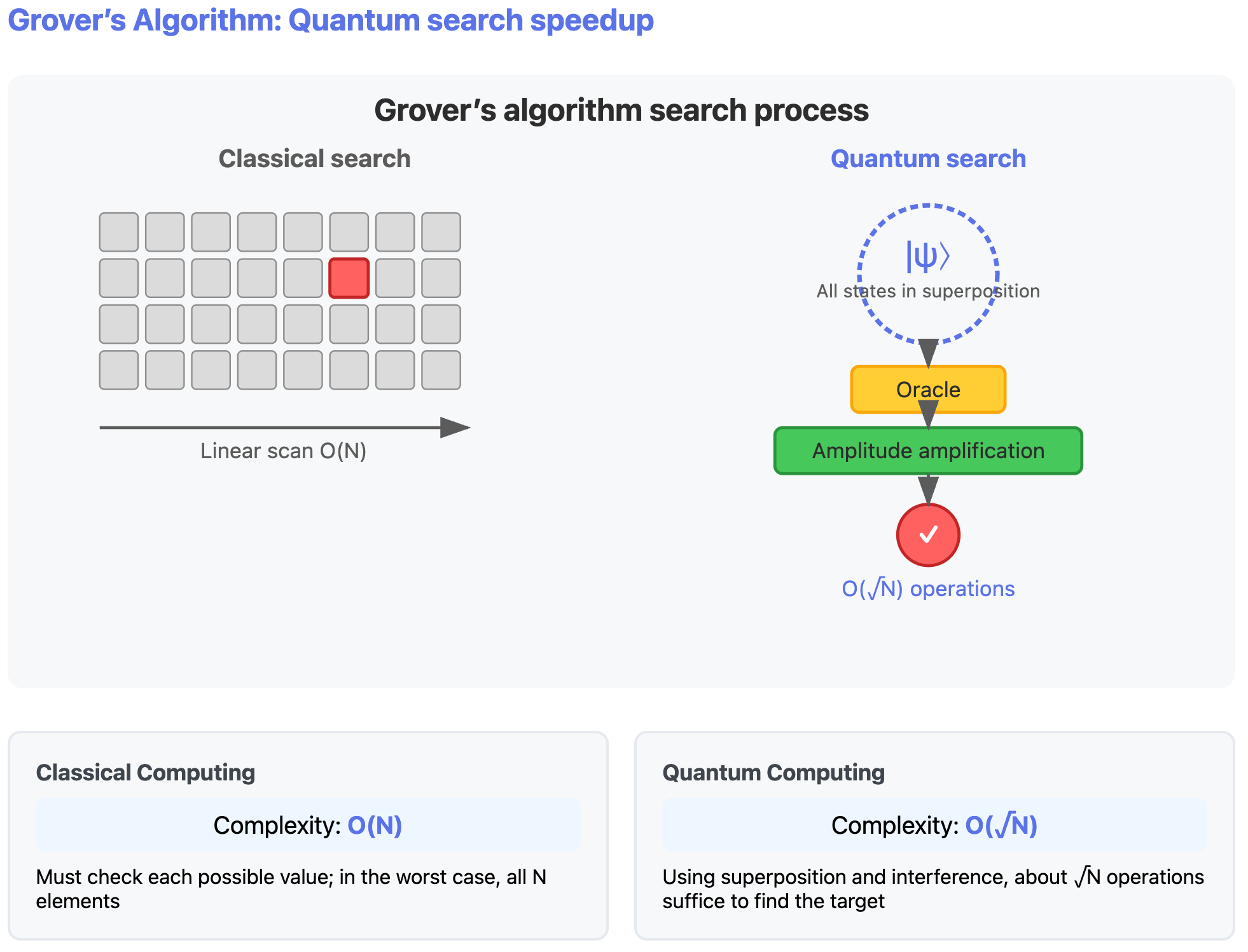
Figure: Grover’s algorithm (schematic).

Cryptographic Application Example: Breaking Hash Functions

Suppose you have a hash function $f(x)$, know a hash value $H$, and want to find some input $x$ satisfying $f(x) = H$. If $x$ is a 4-byte integer (range $2^{32}$), classical computation requires at most $2^{32}$ tries, while Grover’s algorithm only needs approximately $2^{16}$ tries. This acceleration is very useful for password cracking and unordered search.

Similarly, we can also use Grover’s algorithm to accelerate breaking symmetric cryptography like AES.

Shor’s Algorithm: Accelerating Integer Factorization

Difficulty of Classical Integer Factorization

Integer factorization is a classic problem: given a large composite number $N$, find two integers $p$ and $q$ greater than 1 such that $N = p \times q$. When $N$ is the product of two sufficiently large prime numbers, classical computers need to try a large number of possible values, with time complexity growing exponentially. This is the security foundation of RSA encryption: factoring a 2048-bit integer is an almost impossible task.

How Does Quantum Computing Accelerate Integer Factorization?

First, we can transform the integer factorization problem into a “period problem” through number theory knowledge. Shor’s algorithm uses quantum Fourier transform to efficiently extract the period, thereby calculating factors. The core logic is as follows:

Transform into period problem

Choose a random number $a$, calculate $f(x) \equiv a^x \pmod N$. This calculation generates a periodic sequence, such as:

$$ f(0) = 1, f(1) = 3, f(2) = 9, f(3) = 27, f(4) = 9, f(5) = 27, \cdots $$

The sequence repeats every certain length, and this repetition length is the period $r$. After finding this period, we can quickly obtain a factor of $N$, then recursively factorize other factors of $N$.

Quantum Fourier transform extracts period

In classical computation, finding the period requires trying one by one, which is very time-consuming. Quantum computing “simultaneously computes” all possible $x$ through superposition states. By having quantum bits accumulate phases proportional to the period in a series of controlled modular multiplication operations, then using quantum Fourier transform to convert this phase into measurable results, the function’s period $r$ can be extracted in polynomial time.

Calculate factors

Once the period $r$ is known, factors of $N$ can be quickly factorized through simple mathematical formulas. Specifically, factors of $N$ can be obtained by calculating $\text{gcd}(a^{r/2}\pm 1, N)$.

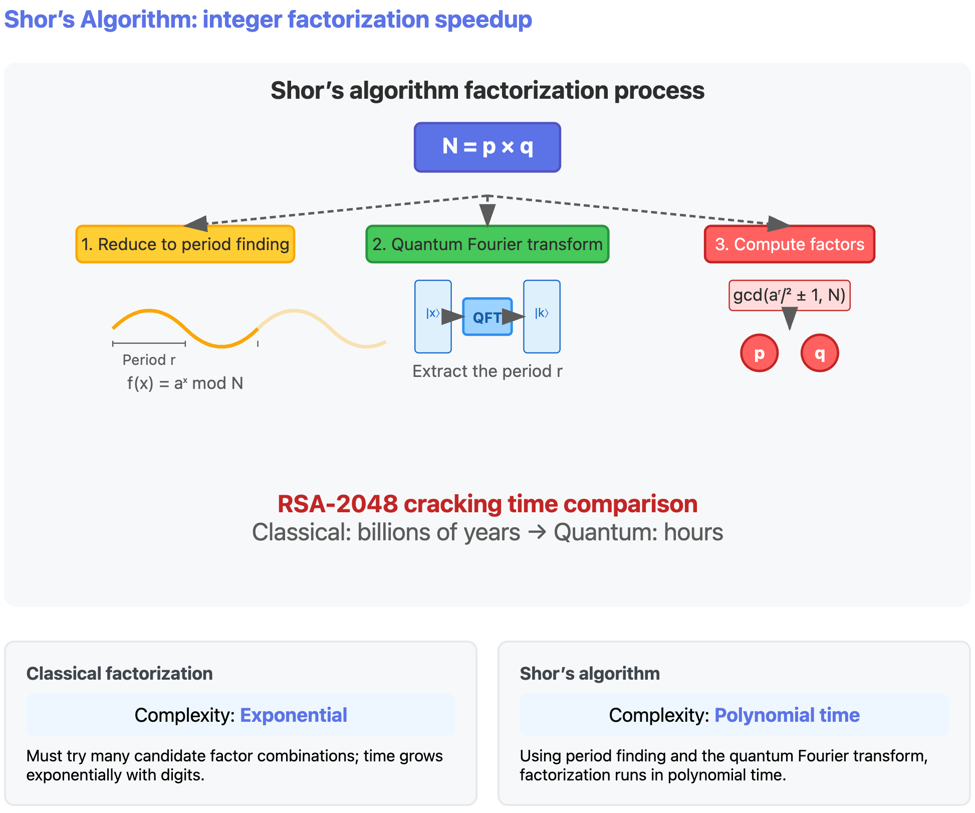
Figure: Shor’s algorithm for factoring RSA (schematic).

Cryptographic Application: RSA Breaking

The security of RSA encryption relies on the difficulty of integer factorization of large numbers. If a classical computer factors a 2048-bit integer, it might take billions of years. Shor’s algorithm can complete the factorization in a few hours, posing a direct threat to modern encryption systems.

Navigation

Part 1: Why Can Quantum Computers Accelerate Computation?

Superposition and Collapse

Quantum Entanglement

Using Superposition and Entanglement to Accelerate Computation

Quantum Computing’s Acceleration Effects on Different Problems

Part 2: How Are Quantum Computers Built?

Physical Implementations of Qubits

Construction Principles of Superconducting Qubits

From Single Qubit to the “System Architecture” of Superconducting Quantum Computing

Quantum Chip

Refrigeration System

Qubit Control System

Quantum Error Correction System

Overall Architecture

Building Quantum Computers Requires Combining Science and Engineering

Part 3: What Challenges Remain in Building a Quantum Computer Capable of Breaking RSA 2048?

Quantum Chip

Wiring Problem

Crosstalk Problem

Device Yield Problem

Hope on the Horizon: Modular Design and Inter-Chip Interconnection

Summary

Refrigeration System

Qubit Control System

Error Correction System

Quantum Computers Capable of Breaking RSA-2048 Will Likely Appear in the 2030s

Appendix 1: Mathematical Expression of Superposition States and Entanglement

Vector Expression of Superposition States and Collapse

Vector Expression of Quantum Entanglement

Wave Function Expression of Quantum States

Relationship Between Wave Function Expression and Vector Expression of Quantum States

Appendix 2: How Quantum Algorithms Threaten Classical Cryptography

Grover’s Algorithm: Accelerating Search Problems

Bottleneck of Classical Search

How Does Quantum Computing Accelerate Search?

Cryptographic Application Example: Breaking Hash Functions

Shor’s Algorithm: Accelerating Integer Factorization

Difficulty of Classical Integer Factorization

How Does Quantum Computing Accelerate Integer Factorization?

Cryptographic Application: RSA Breaking

References

- Beckman, David, et al. “Efficient networks for quantum factoring.” Physical Review A 54.2 (1996): 1034.
- Grover, Lov K. “A fast quantum mechanical algorithm for database search.” Proceedings of the twenty-eighth annual ACM symposium on Theory of computing. 1996.
- Shor, Peter W. “Algorithms for quantum computation: discrete logarithms and factoring.” Proceedings 35th annual symposium on foundations of computer science. Ieee, 1994.
- Nielsen, Michael A., and Isaac L. Chuang. Quantum computation and quantum information. Cambridge university press, 2010.
- Gidney, Craig. “How to factor 2048 bit RSA integers with less than a million noisy qubits.” arXiv preprint arXiv:2505.15917 (2025).
- Gidney, Craig, and Martin Ekerå. “How to factor 2048 bit RSA integers in 8 hours using 20 million noisy qubits.” Quantum 5 (2021): 433.
- Krinner, Sebastian, et al. “Engineering cryogenic setups for 100-qubit scale superconducting circuit systems.” EPJ Quantum Technology 6.1 (2019): 2.
- Kjaergaard, Morten, et al. “Superconducting qubits: Current state of play.” Annual Review of Condensed Matter Physics 11.1 (2020): 369-395.
- Bruzewicz, Colin D., et al. “Trapped-ion quantum computing: Progress and challenges.” Applied physics reviews 6.2 (2019).
- Browaeys, Antoine, and Thierry Lahaye. “Many-body physics with individually controlled Rydberg atoms.” Nature Physics 16.2 (2020): 132-142.
- Burkard, Guido, et al. “Semiconductor spin qubits.” Reviews of Modern Physics 95.2 (2023): 025003.
- Wang, Jianwei, et al. “Integrated photonic quantum technologies.” Nature photonics 14.5 (2020): 273-284.
- Castelvecchi, Davide. “IBM releases first-ever 1,000-qubit quantum chip.” Nature 624.7991 (2023): 238-238.
- “Postquantum Cryptography: The Time to Prepare Is Now!” Gartner Research(2024)
- Joseph, David, et al. “Transitioning organizations to post-quantum cryptography.” Nature 605.7909 (2022): 237-243.
- Fowler, Austin G., et al. “Surface codes: Towards practical large-scale quantum computation.” Physical Review A—Atomic, Molecular, and Optical Physics 86.3 (2012): 032324.
- “Quantum error correction below the surface code threshold.” Nature 638, no. 8052 (2025): 920-926.